2D Curve Drawing (NURBS)
Site Map Feedback
Curve Drawing
Up Buttons Circles Curves Lines
Understanding curve-drawing is easy if the idea is grown from basic principles...
Ready for a journey?

Linear Bezier spline:

Imagine two 3D points in space which are not coincident.
The shortest journey from one point to the other is a straight line.
When rendering a line this journey is performed, and pixels are set as required - so the journey itself is important.
Consider a measure of the journey's progress to be a percentage of the total journey.
When you're half way to the destination point, that's 50% of the journey done and 50% left to do.
This is the first principle used in curve-drawing, but rather than a percentage going from 0 to 100, the journey goes from 0 to 1.
Zero means you're at the start point, 0.5 means half way, 1.0 means you're at the end point.
This is a common way of dealing with lines, called the "Parametric Representation" as discussed on the Mapping page.
Rather than thinking of two points, think of one point and a vector describing the journey (a Position vector).
V = EndPoint - StartPoint
t is conventionally used to represent the journey position.
P(t) = StartPoint + t * V, 0<=t<=1
As t moves from 0 to 1 it traces out the line from the start point to the end point.

Quadratic Bezier spline:

Quadratic Bezier Curve Drawing To extend this idea to trace curves, add more points.
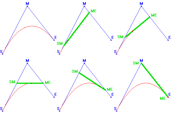
So imagine three points (in triangle formation), a start(S), middle(M) and end(E), joined by two lines.
The Middle point here is considered to be a Control Point: its position defines how curved the line will be.
Now add a line from the mid-point of S-M (call this new point SM) to the mid-point of M-E (call this new point ME)...
The triangle is starting to look like a curve from the start point to the end point.
Now imagine that this third line is mobile instead of being fixed to the mid-points of the other two lines:
It's going on a journey.
The end (SM) which joins S-M will begin at S and travel to M.
The end (ME) which joins M-E will begin at M and travel to E.
Trace a line with a pencil which is going to travel along the moving line from SM to ME.

Since all the lines may be different lengths, use the same journey ratio (t) for all the lines.
So, at the beginning, t=0, the mobile line will be joined to S and E and the pencil will be at SM.
Half way through (t=0.5) the mobile line will joined to the mid-point of S-M and the mid-point of M-E, and the pencil will be at the mid-point of SM-ME (the mobile line).
At the end (t=1) the mobile line will be joined to M and E and the pencil will be at ME.
Obviously the length of the mobile line will be changing, and the speed of the moving points will all be different if the two static lines are different lengths.
P(t)=(1-t)*(1-t)*P1 + 2*(1-t)*t*P2 + t*t*P3
This is a linear interpolation between linear interpolations between control points (deCasteljau algorithm).

Cubic Bezier spline:

So, if you add another control point you'll have three lines and you can do the same thing but to another level:
A linear interpolation between linear interpolations between linear interpolations between control points!
This is the most common Bezier used.
The endpoints have to be points, but the internal control points can just be vectors.
You can scale or transform a Bezier simply by scaling or transforming its control points (Affine Invariance).
If all the control points form a straight line, the curve also forms a line.
A Bezier curve is tangent to the first and last segments of the control polygon.
For Beziers, n is used to denote the "Degree" of the curve which is the same as the number of lines between Control Points (which is Control Points-1).
The "Order" is the same as the number of Control Points.
It's called Order because it represents the order of the polynomial that is solved to make the journey.
The higher the order, the more processing required - so high-order Beziers are bad.

B-spline:

Imagine two Bezier Splines which are joined to each other tangentially.
The Endpoint of the first Curve will have the same values as the start-point of the second Curve.
For the Curves to meet tangentially, the Control Point vectors will be exact opposites.
A Cubic B-spline is made of a string of Cubic Beziers which join tangentially.
To create a Cubic B-spline you need 4 Control Points for the first Bezier, but the next one only requires one extra Control Point (its End Point) because the Tangential Constraint defines all the other Control Points.
Notice that now, the Order is 3 (Cubic) but that there are two Beziers which can describe a more complex curve.
The start and end of each Bezier is called a "Knot" as if the B-spline were string of Beziers tied together.
To create a closed loop you need only make the last "Degree" Knot values the same as the first, eg: {1,2,3,4,1,2,3}
In a B-spline each control point is associated with a Basis Function which is given by a recursive equation and returns values from 0 to 1.
A Basis Function is a polynomial of order "Order" - it is a weighting, representing the closeness to the Control Point.
The shapes of the Basis Functions are determined entirely by the relative spacing between the Knots.
At any t point you are dealing with the nearest Bezier.
This is the same as saying:
At any t point, B-splines depend on the same number of nearest Control Points as the Order.
"Uniform Knot Vectors" means the Knot values are equally spaced.
"Open Uniform Knot Vectors" are Uniform Knot Vectors which have the same number of equal Knot values at each end as the Order. This makes the B-spline start at the first Control Point and end at the last.
"Non-uniform Knot Vectors" are the general case.
Increasing the Order increases smoothness of a curve and tends to move the curve further from its control polygon.

Non-Uniform Rational B-splines (NURBS):

Since the shapes of the Basis Functions are determined entirely by the relative spacing between the Knots, it is useful to add one more weight for each Control Point which can be set independently of everything else.
NURBS use a 0 to 1 multiplier for each control point.
The weight value determines the intersection location of the curve with the Control Point polygon.
There are two different conventions for representing the control points in terms of their 4D coordinates (x,y,z,w):
"Homogeneous", in which the coordinates represent the point's position in 4D space. Thus the point's 3D position is (x/w, y/w, z/w).
"Weighted Euclidean", in which the coordinates are already considered to have been divided. Thus the first three components (x,y,z) directly represent the point's position in 3D space and the fourth w represents its weight.

NURBS for Conic Section:

A Conic Section is the result of intersection of a Cone with a Plane.
The angle at which the Plane intersects the Cone determines whether the resulting curve is a Circle, Ellipse, Parabola or Hyperbola.
Conic curves may be represented using quadratic NURBS (2 Lines, Order=3) with 6 open uniform Knots [0 0 0 1 1 1]:
Parabola (The weight of the Inner Control Point is 1)
Hyperbola (The weight of the Inner Control Point is 4)
Ellipse (The weight of the Inner Control Point is 1/4)
The following method can be used to construct a circular arc of quadratic NURBS:
The legs of the control triangle are of equal length (i.e. it is isosceles).
The chord connecting the first and the last control points meets each leg at an angle f equal to half the angular extent of the arc.
The weight of the Inner Control Point is cos(f).
The open uniform knot vector is [0,0,0,1,1,1].


THIS SOFTWARE IS PROVIDED BY THE COPYRIGHT HOLDERS AND CONTRIBUTORS 'AS IS' AND ANY EXPRESS OR IMPLIED WARRANTIES, INCLUDING, BUT NOT LIMITED TO, THE IMPLIED WARRANTIES OF MERCHANTABILITY AND FITNESS FOR A PARTICULAR PURPOSE ARE DISCLAIMED. IN NO EVENT SHALL THE REGENTS OR CONTRIBUTORS BE LIABLE FOR ANY DIRECT, INDIRECT, INCIDENTAL, SPECIAL, EXEMPLARY, OR CONSEQUENTIAL DAMAGES (INCLUDING, BUT NOT LIMITED TO, PROCUREMENT OF SUBSTITUTE GOODS OR SERVICES; LOSS OF USE, DATA, OR PROFITS; OR BUSINESS INTERRUPTION) HOWEVER CAUSED AND ON ANY THEORY OF LIABILITY, WHETHER IN CONTRACT, STRICT LIABILITY, OR TORT (INCLUDING NEGLIGENCE OR OTHERWISE) ARISING IN ANY WAY OUT OF THE USE OF THIS SOFTWARE, EVEN IF ADVISED OF THE POSSIBILITY OF SUCH DAMAGE.